Language Modeling by Estimating the Ratios of the Data Distribution

Modern large language models (like ChatGPT) learn to generate new samples by modeling the data distribution of natural text. However, the underlying methodology has largely remained stagnant over the last century: although different architectures have been developed, models are all based on autoregressive modeling (i.e. next token prediction). In this blog post, I will talk about our work on Score Entropy Discrete Diffusion models, an alternative probablistic modeling technique that achieves highly competitive performance (at the scale of GPT-2) while introducing distinct algorithmic benefits. Our empirical results challenge the longstanding dominance of autoregressive modeling and can potentially pave the way for an alternative class of language models built from radically different principles.

Introduction

At the core of modern generative AI systems lies the field of probabilistic modeling. The idea behind probabilistic modeling is surprisingly straightforward and consists of three steps:

1. Collect a dataset \(x_1, x_2, \dots, x_n\) which we assume has been sampled i.i.d. from our underlying data distribution \(p_{\mathrm{data}}\).

2. Learn a parameterized density \(p_{\theta}\) (often using a neural network) such that \(p_{\theta} \approx p_{\mathrm{data}}\). For example, we could use our dataset to minimize the negative log likelihood loss: \(\begin{equation} \mathbb{E}_{x \sim p_\mathrm{data}}[-\log p_\theta(x)] \approx \frac{1}{n} \sum_{i = 1}^n -\log p_\theta(x_i) \end{equation}\)

3. Use \(p_\theta\) to generate new samples. Bonus points if we can sample conditionally \(p_\theta(\cdot \vert c)\) (where \(c\) is something like a prompt, desired property, etc…).

For a data domain such as natural language (which this blog post focuses on), things seem like they should be easy. In particular, our data is discrete, meaning that the support of \(p_{\mathrm{data}}\) lies on a finite set \(\mathcal{X} = \{1, \dots, \vert\mathcal{X}\vert\}\). For the simple examples we might find in a standard undergraduate probability textbook, we can directly learn the probabilities of each element:

A probability density function for the sum of two dice rolls. One could directly learn the values of $p_\theta(2)$, $p_\theta(3)$, ..., $p_\theta(12)$ with a maximum likelihood estimator given some samples.

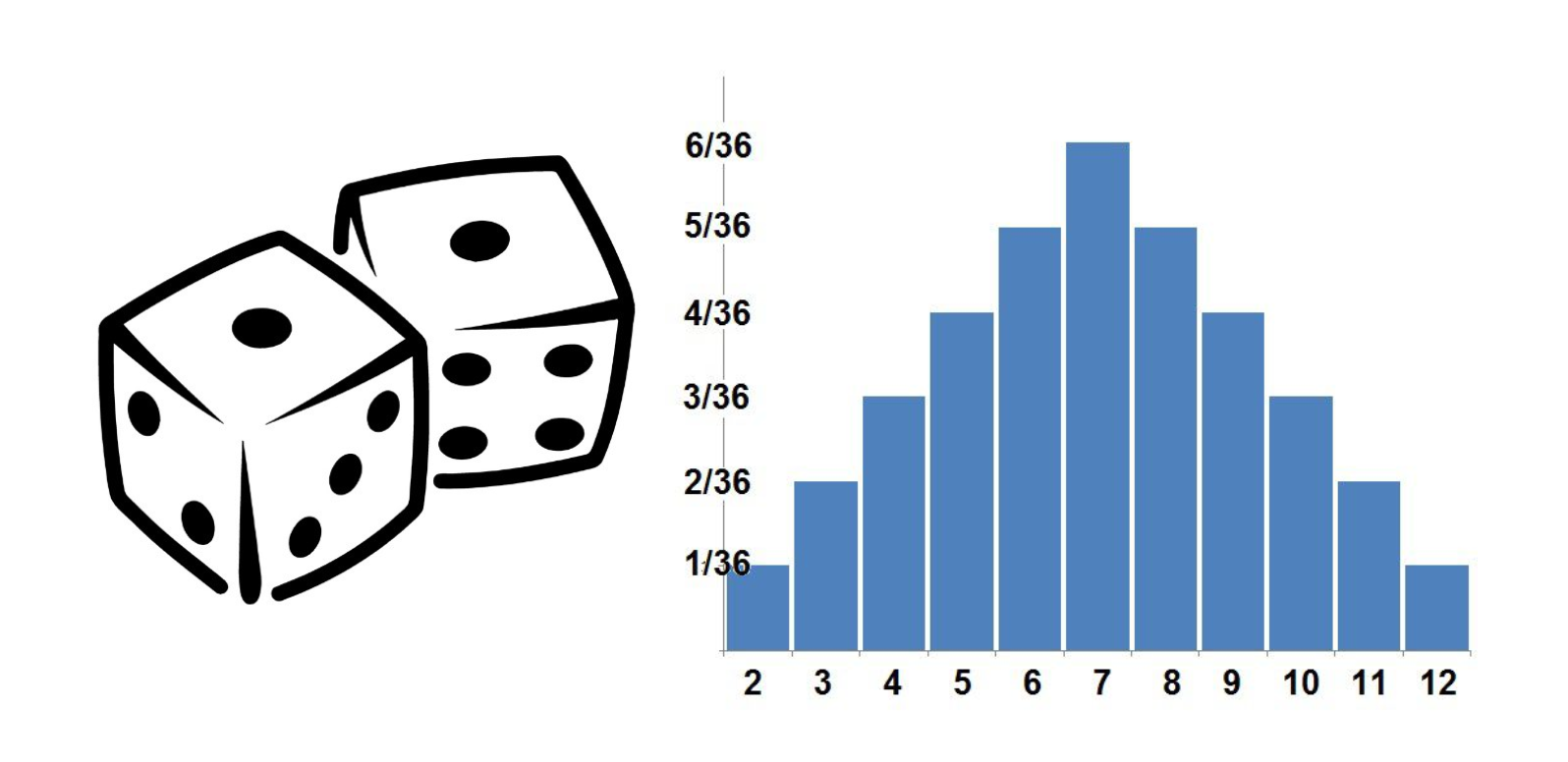
Unfortunately, real world datasets are much more complex than this. For something like natural language, we are working with something like the Library of Babel, where all possible combinations of characters must be analyzed. This makes things quite a bit more challenging.

For natural language, we need to calculate $p_\theta$ for exponentially many inputs.

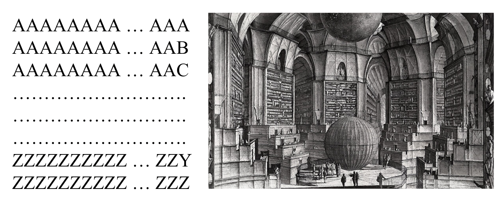
To overcome this challenge, we use a parameterized model (like a neural network) to map values to probabilities \(p_\theta: \mathcal{X} \to \mathbb{R}\), but our troubles are not over yet. In particular, constructing a valid probability density \(p_\theta\) requires two mathematical conditions:

\[\begin{equation} p(x) \ge 0 \quad \text{ and } \quad \sum_{x \in \mathcal{X}} p(x) = 1 \end{equation}\]

Since neural networks \(f_\theta\) (by construction) output general values, enforcing these conditions requires additional constraints. For example, one could build an energy based model:

\[\begin{equation} p_\theta(x) = \frac{e^{f_\theta(x)}}{Z} \quad \text{ where } \quad Z = \sum_{x \in \mathcal{X}} e^{f_\theta(x)} \end{equation}\]

But, for this type of parameterization, computing \(Z\) is near-impossible due to the curse of dimensionality (forcing one to rely on crude approximations). For example, for something like GPT-2, computing \(Z\) would requiring evaluating \(p_\theta\) for all \(50257^{1024}\) different possible input sentences (this is a number far greater than the number of atoms in the known universe).

Autoregressive Modeling

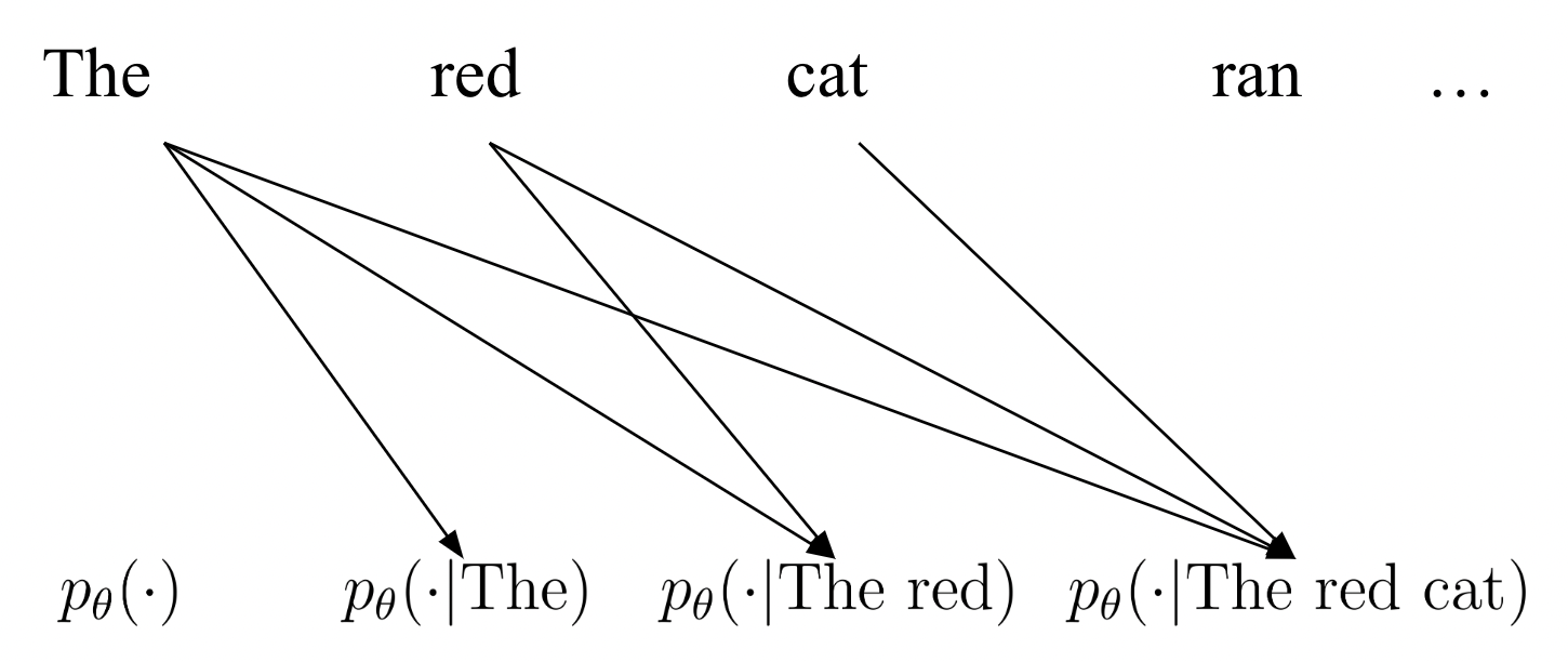
Luckily for us, there is a way to make this problem tractable. In almost all practical applications, our data support \(\mathcal{X}\) is highly structured, factorizing into a product set \(\mathcal{X} = \{1, \dots, N\}^d\) so that elements are given by \(\mathbf{x} = x^1 x^2 \dots x^d\). For real world examples, this would break down a sentence (“The red dog ran.”) into its constituent parts (“The”, “red”, “dog”, “ran”, “.”). Because we instead model sequences \(x^1 x^2 \dots x^d\), we can decompose using the probablistic chain rule:

\[\begin{equation} p_{\mathrm{data}}(x^1 x^2 \dots x^d) = p_{\mathrm{data}}(x^1) p_{\mathrm{data}}(x^2 \vert x^1) \dots p_{\mathrm{data}}(x^d \vert x^1 \dots x^{d - 1}) \end{equation}\]

This motivates autoregressive modeling, which instead seeks to learn each component probability \(p_\theta(x^i \vert x^1 \dots x^{i - 1}) \approx p_{\mathrm{data}}(x^i \vert x^1 \dots x^{i - 1})\). As a result, this is often colloquially called next token prediction. Compared with the naive approach, this is extremely scalable since each component probability’s normalizing constant consists of \(N\) terms. Furthermore, sampling is easy (just sample \(x_1\), then \(x_2\), etc…), and you can even control the process by feeding in a fixed prefix to complete.

Autoregressive modeling setup: a neural network learns to predict the next token given the previous ones.

Why are There (Almost) No Alternatives?

Autoregressive modeling is perhaps the simplest workable approach imaginable. Yet, despite the numerous advances in the field of generative models, no competitive alternative has been presented for discrete data. Ultimately, the core obstacle is actually the discrete nature of the data itself. Rather than simplifying our space, this structure breaks the fundamentals of calculus, which, incidentally, our neural networks rely on.

To illustrate this point, consider a classic GAN training setup. For image generation, a GAN first generates an image from random noise and then uses a discriminator to penalize deviations, allowing for gradients to backpropagate to the generator.

A GAN trained to produce images. We can feed generations into a discriminator to train our generator $f_\theta$.

Now, suppose the GAN generates discrete text. While one could define a generator and discriminator using similar principles, a fundamental error occurs. Unlike images, which are continuous and thus enable backpropagation to compute gradients, text is a discrete value which can’t be differentiated. As such, computing the gradient learning signal for the generator is a cumbesome process (often relying on crude approximations and/or estimations).

A GAN trained to generate text. While we can build a generator and discriminator, the discrete nature of text makes it very challenging to update to our generator.

Other approaches largely run into similar problems, leaving autoregressive modeling as the only viable contender. Without fundamental advancements to the core probabilistic framework, generative models for discrete data have instead progressed by repeatedly iterating on the neural network architecture. In particular, modern methods largely revolve around the transformer model, which simultaneously evaluates \(p_\theta(x^1), \dots, p_\theta(x^d \vert x^1 \dots x^{d - 1})\) to enable fast, scalable training. This approach has led to the creation of large language models (such as ChatGPT, LLAMA, Gemini), which dominate the landscape of artifical intelligence.

Score Entropy Discrete Diffusion Models

As the field of autoregressive transformers reaches a natural maturity, many have started to believe that more data, better hyperparameters, and larger architectures are all you need for AGI. Yet, there are still fundamental shortcomings of this autoregressive framework

1. Famously, AI Godfather Yann Lecun has argued that autoregressive transformers are “doomed”, as generation “drifts” from the data distribution and causes the model to diverge during sampling. In pratice, such phenomena must be aggressively curtailed with distribution annealing hacks (disallowing low probability tokens at the expense of diversity), especially at smaller scales.
2. Furthermore, sampling is highly iterative, which is not ideal for our highly optimized GPU systems that are built for parallel computation.
3. Lastly, these models complete from left to right, making it very difficult to perform several control tasks (like infilling text given a prefix and a suffix).

These shortcomings motivate us to define an alternative probabilistic model, which we coin the Score Entropy Discrete Diffusion (SEDD) model.

Concrete Scores as an Alternative Probabilistic Model

We saw that the main failure of energy based models was the computation of the normalizing constant \(Z\). If we could avoid computing the \(Z\), our approach would greatly simplify. So, instead of directly modeling \(p_\theta(x)\), we instead model the ratios \(\frac{p_\theta(y)}{p_\theta(x)}\), eliminating \(Z\)

\[\begin{equation} \frac{p_\theta(y)}{p_\theta(x)} = \frac{e^{f_\theta(y)} / Z}{e^{f_\theta(x)} / Z} = \frac{e^{f_\theta(y)}}{e^{f_\theta(x)}} \end{equation}\]

These ratios collectively form a quantity known as the concrete score, which can directly be modelled by a neural networkSince the positivity condition is easy to enforce with an exponential, we ignore it in our setup \(s_\theta(x)_y \approx \frac{p_{\mathrm{data}}(y)}{p_{\mathrm{data}}(x)}\). In particular, this quantity is the categorical equivalent of the famous score function \(\nabla_x \log p\) in continuous space A score function is given by $\nabla_x \log p = \frac{\nabla_x p}{p(x)}$. Since gradients become finite differences in discrete space, the equivalent to a score function would be $\frac{p(y) - p(x)}{p(x)} = \frac{p(y)}{p(x)} - 1$, which is the concrete score minus one., which motivates many of our developed methods.

The score function $\nabla_x \log p$ (left) intuitively "points" to higher density areas in continuous space, something that the concrete score $\frac{p_t(y)}{p_t(x)}$ (right) generalizes for discrete spaces.

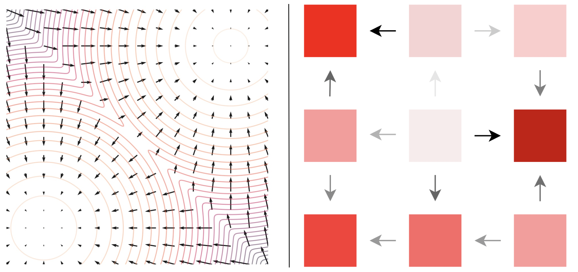
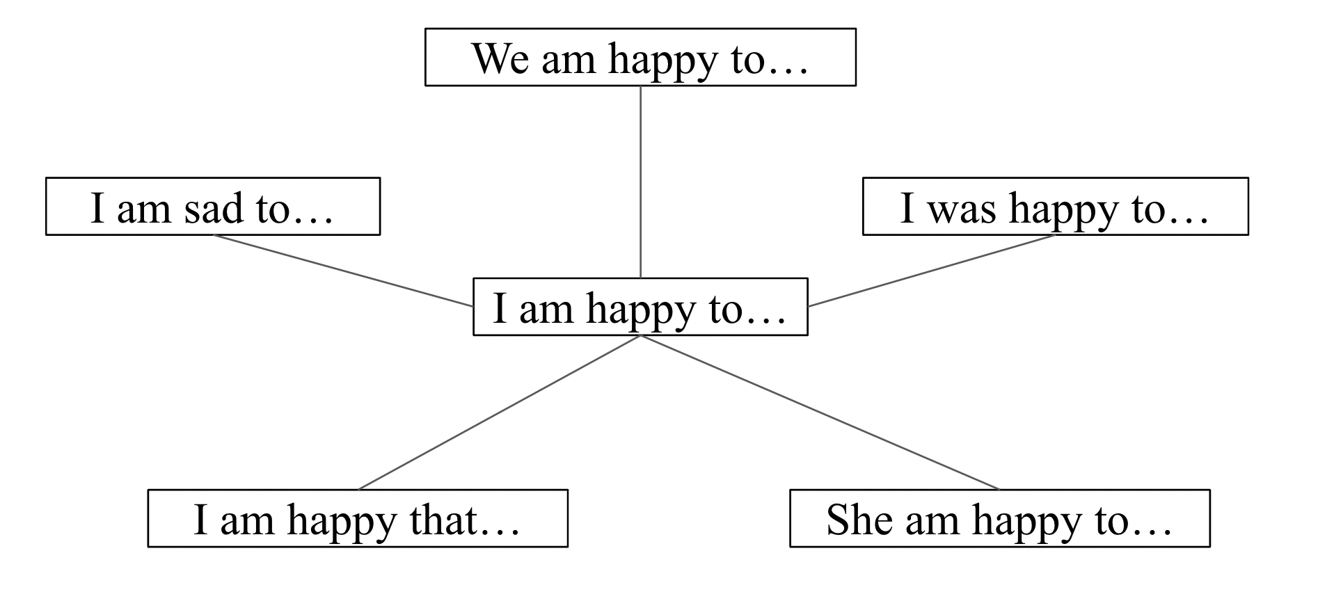
Importantly, we wrote out our neural network approximation as \(s_\theta(x)_y\), emphasizing that a single network evaluation \(s_\theta(x)\) should evaluate all ratios with denominator \(p_{\mathrm{data}}(x)\). If we model the ratio for every possible \(y\), we would have \(N^d\) items (again, computationally intractable), so we sparsify and only model “relevant” ratios based on whether \(y\) is “close” to \(x\). These relevant positions will be denoted as \(y \sim x\) (symbolizing that \(y\) is a neighbor of \(x\) in graph theory), and, for this blog post, will be something like all sentences \(y\) that differ from \(x\) at one position (or Hamming distance \(1\)):

We model the probability ratios between neighboring sentences. In this case, these differ by exactly at one position.

Learning Concrete Scores with Score Entropy

With our neural network \(s_\theta\), we now formulate a training loss for learning the concrete scores. Here, we draw inspiration from the cross entropy loss function (which is built for learning positive probabilistic quantities)

\[\begin{equation}\mathbb{E}_{y \sim p_\mathrm{data}}[-\log p_\theta(y)] = - \sum_{y} p_{\mathrm{data}}(y) \log p_\theta(y)\end{equation}\]

to define the score entropy:

\[\begin{equation} \sum_{y \sim x} s_\theta(x)_y - \frac{p_\mathrm{data}(y)}{p_\mathrm{data}(x)} \log s_\theta(x)_y \end{equation}\]

Score entropy generalizes cross entropy by allowing one to learn arbitarary \(\frac{p_\mathrm{data}(y)}{p_\mathrm{data}(x)}\), not just \(p_\mathrm{data}(y)\) (which must sum to \(1\)).In particular, cross entropy is recovered we constrain $s_\theta(x)_y$ to sum to $1$ over all $y \sim x$ (removing the first term since it sums to a constant $1$ and resulting in cross entropy scaled down by a factor of $p_\mathrm{data}(x)$). Notably, it also forms a nice, convex loss curve that correctly accounts for the positivity of \(s_\theta\) (not letting it go negative).

Our score entropy forms a convex loss that has a log-barrier at $0$ for all ground truth $\frac{p_\mathrm{data}(y)}{p_\mathrm{data}(x)}$.

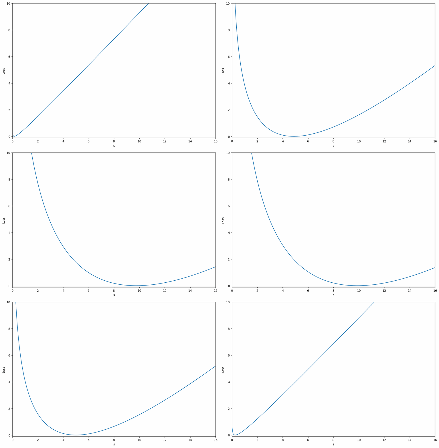
In practice, we can combine the score entropy loss for all values of \(x\) using our \(p_{\mathrm{data}}\), allowing us to approximate it with Monte Carlo sampling

\[\begin{align} \mathbb{E}_{x \sim p_\mathrm{data}} &\left[\sum_{y \sim x} s_\theta(x)_y - \frac{p_\mathrm{data}(y)}{p_\mathrm{data}(x)} \log s_\theta(x)_y\right] \\ &= \frac{1}{n} \sum_{i = 1}^n \left[\sum_{y \sim x_i} s_\theta(x_i)_y - \frac{p_\mathrm{data}(y)}{p_\mathrm{data}(x_i)} \log s_\theta(x_i)_y\right] \end{align}\]

While score entropy is a nice theoretical construct, it requires too much prior information to work. In particular, if we already knew \(\frac{p_\mathrm{data}(y)}{p_\mathrm{data}(x)}\) (which we regress on in our loss), then we wouldn’t have to learn it in the first place!

Following standard techniques in score matching, we can rework our loss (deriving a tractable equivalent) with some math. For example, if we assume that our data distribution \(p_{\mathrm{data}}\) arises as a perturbation of a base density \(p_0\) (i.e. \(p_{\mathrm{data}}(x) = \sum_{y} p(x \vert y) p_{0}(y)\)), then our loss is equivalent to the following denoising score entropy loss

\[\begin{equation}\label{eqn:dse} \mathbb{E}_{x_0 \sim p_0, x \sim p(\cdot \vert x_0)} \left[\sum_{y \sim x} s_\theta(x)_y - \frac{p(y | x_0)}{p(x | x_0)} \log s_\theta(x)_y\right] \end{equation}\]

In particular, this replaces the unknown \(\frac{p_{\mathrm{data}}(y)}{p_{\mathrm{data}}(x)}\) with the known transition ratio \(\frac{p(y \vert x_0)}{p(x \vert x_0)}\), enabling tractable optimization.

Generating Samples with Concrete Scores

While the previous section showed that we can use score entropy to learn the concrete score from data (corresponding to learning the probabilistic model), we still don’t know how to generate samples. To do this, we will borrow the core idea from diffusion models and use our learned concrete score to iteratively denoise random values into data points.

A diffusion model iteratively "denoises" a noisy image by reversing the injection of Gaussian noise.

To do this, we must first define what a “adding noise” to a discrete text sample means. While for continuous space, such a perturbation comes about naturally by adding Gaussian noise, discrete spaces are forced to “jump” directly between different elements.

We perturb a discrete text sequence by randomly mutating each element of the sequence independently.

Mathematically, such evolutions are known as discrete diffusion processes. We can describe such a process with a differential equation that evolves our “clean” data distribution \(p_0\) to increasingly noisy distributions \(p_t\):

\[\begin{equation} \frac{dp_t}{dt} = Q p_t \quad \quad p_0 = p_{\mathrm{data}} \end{equation}\]

Remember that, since our support is discrete, \(p_t\) is just a vector, so \(Q\) is a matrix that determines the diffusion evolution. Since \(p_t\) is extremely high dimensional, we can’t measure it, but we can simulate the evolution of an element according to \(p_t\). Intuitively, the columns of \(Q\) control how likely one “jumps” from state to state: for small \(\Delta t\) steps, we have a jumping strategy of

\[\begin{equation} p(x_{t + \Delta t} = a \vert x_t = b) \approx \delta_b(a) + Q(a, b) \Delta t \end{equation}\]

In particular, we see that \(Q(a, b)\) is a measurement of how likely \(a\) is to jump to \(b\). In practice, \(Q\) could be something like

\[\begin{equation} \begin{bmatrix} -3 & 1 & 1 & 1 \\ 1 & -3 & 1 & 1 \\ 1 & 1 & -3 & 1\\ 1 & 1 & 1 & -3\end{bmatrix} \end{equation}\]

which would mean every two elements are equally likely. In particular, since we work with sequences, we choose to perturb at each position independently so we don’t destory information entirely.

Importantly, as \(t \to \infty\), \(p_t\) approaches some noise distribution \(p_{\mathrm{noise}}\) (which is easy to sample from, such as a random value in each position). We can derive a reverse diffusion process that reverse the density from some \(p_T \approx p_{\mathrm{noise}}\) back to our \(p_0\):

\[\begin{equation} \frac{dp_{T - t}}{dt} = \overline{Q}_{T - t} p_{T - t} \quad \overline{Q}_t(x, y) = \frac{p_t(y)}{p_t(x)} Q(y, x) \end{equation}\]

Here, we can reconstruct the jumping strategy but in reverse, seeing that this process intuitively pushes towards higher probability regions:

\[\begin{equation} p(x_{t - \Delta t} = a \vert x_t = b) \approx \delta_b(a) + \frac{p_t(a)}{p_t(b)}Q(b, a) \Delta t \end{equation}\]

The \(\frac{p_t(y)}{p_t(x)}\) are unknown, but we can learn them using score entropy! In fact, our denoising score entropy (Equation \(\ref{eqn:dse}\)) can readily be applied with our diffusion setup, since each \(p_t\) comes about by perturbing the base \(p_0\) (i.e. \(p_t(x) = \sum_{y} p_{t \vert 0}(x \vert y) p_0(y)\)), with the transition densities \(p_{t \vert 0}\) arising as functions of \(Q\).

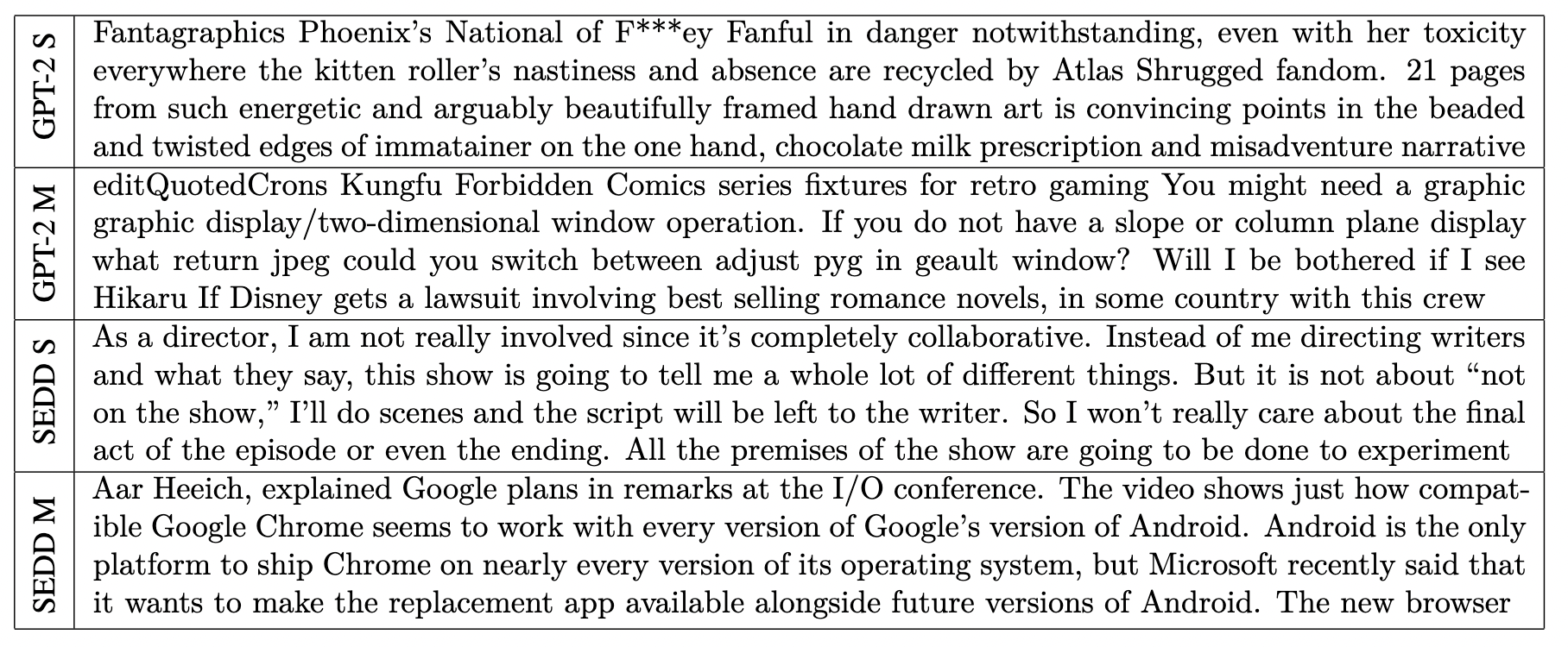
With such a learned neural network \(s_\theta(x, t)_y \approx \frac{p_t(y)}{p_t(x)}\), we can generate samples by drawing \(x_T \sim p_T\) and simulating the above process (with \(s_\theta\) replacing our unknown ratio). By doing so, we are able to generate high quality text:

Our model learns to iteratively denoise a sample into text, generating from a purely random input.

When compared with autoregressive models, our approach can use complete global context during generation, resulting in better overall generation. In particular, autoregressive models like GPT-2 do indeed “drift”, destabilizing performance for full length generations, while our approach maintains a coherent global structure and results in significantly better quality.

Some generated samples from GPT-2 and SEDD across small and medium sizes. SEDD is able to consistently generate high quality text even at smaller scales, while baseline GPT-2 (autoregressive) models struggle.

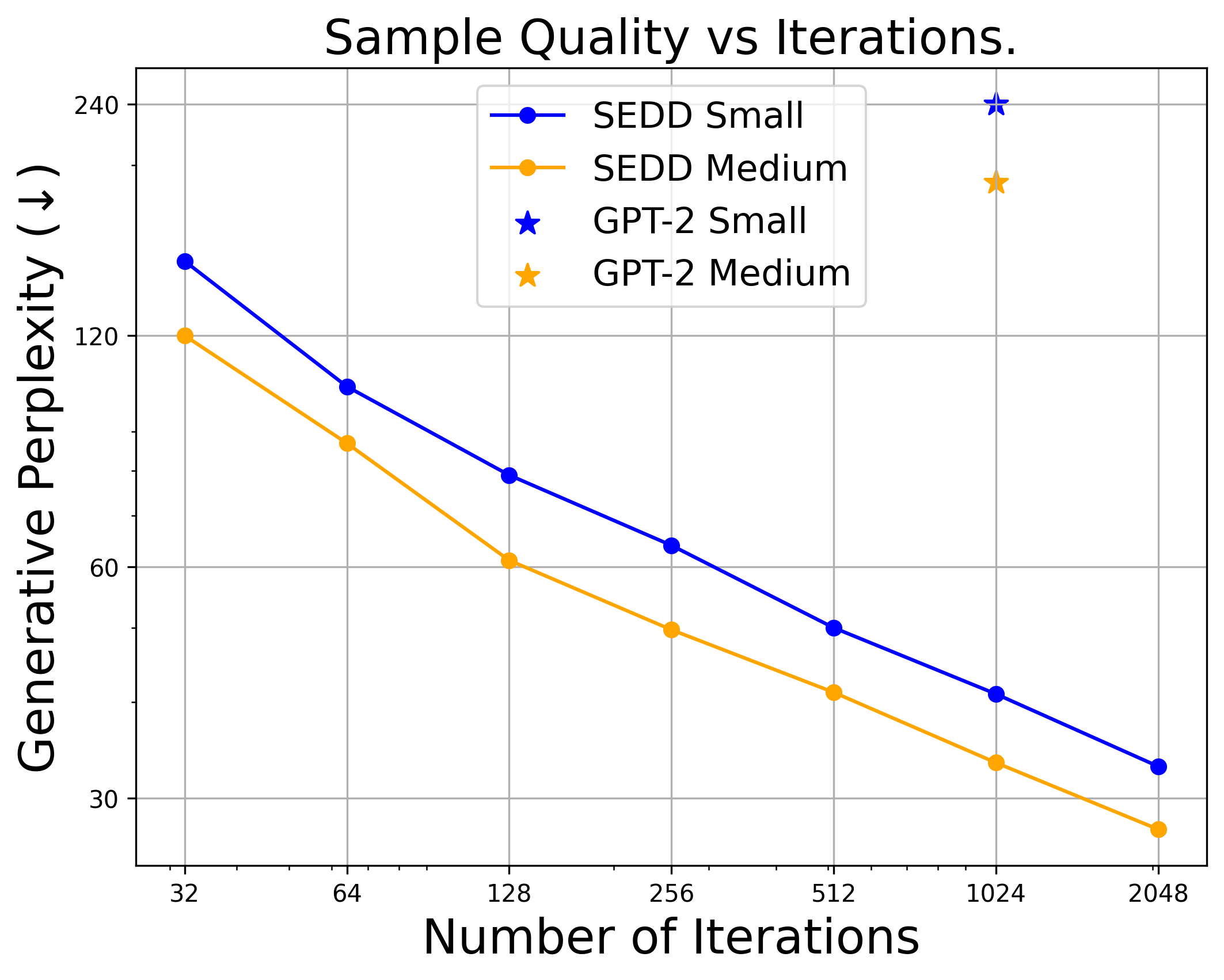
Furthermore, we can trade off compute for quality, something that isn’t possible for autoregressive models, enabling us to generate good samples with far fewer iterations. By graphing out the generation quality vs number of sampling steps, we can readily see a direct performance tradeoff.

Sample quality versus iterations. Our SEDD samples are significantly better (lower generative perplexity metric) when compared with the corresponding GPT-2 samples. Additionally, the number of sampling iterations forms a log-log tradeoff with generation quality.

One other cool thing is that we can prompt our generation similar to autoregressive generation. In fact, this is even more flexible, since we can prompt from any position, not just from left to right. The setup is very simple: given prompt tokens at \(\Omega\), we simply treat these as constants that we don’t change during the sampling process.

For an arbitrary prompt, we can reuse our score function $s_\theta$ to sample conditionally by simply simulating the same sampling procedure but only changing the non-prompt tokens.

While naive, this is actually principled! Suppose we are given an input \(c\) at indices \(\Omega\) and wish to fill in the remaining indices \(\overline{\Omega}\). We would still generate by reversing a discrete diffusion process, but the only difference is now we need conditional concrete scores \(\frac{p_t(\cdot \vert \Omega = c)}{p_t(\cdot \vert \Omega = c)}\). However, we can decompose these by bayes rule:

\[\begin{equation} \hspace{-2cm}\frac{p_t(\overline{\Omega} = z | \Omega=c)}{p_t(\overline{\Omega} = y | \Omega=c)} = \frac{p_t(\overline{\Omega} = z \cap \Omega = c) / p_t(\Omega = c)}{p_t(\overline{\Omega} = y \cap \Omega = c) / p_t(\Omega = c)} = \frac{p_t(\overline{\Omega} = z \cap \Omega = c)}{p_t(\overline{\Omega} = y \cap \Omega = c)} \end{equation}\]

In particular, the conditional and unconditional scores are the same, so we can reuse our base score netork \(s_\theta\) to model the conditional ratios.

When we test with a variety of prompting schemes, our model is capable of generating high quality text, matching the best autoregressive sampling strategies using both standard (left to right) and nonstandard (fill in the middle) prompting. Note that neither of these prompting strategies are explicitly learned, making our results zero-shot.

Method	MAUVE Score (↑)
GPT-2 w/ nucleus sampling	0.955
SEDD w/ standard prompting	0.957
SEDD w/ infilling prompting	0.942

Evaluating Likelihoods of the Generative Process

For language models, one important indicator of performance is perplexity, which is a function of the model’s log probability.

\[\begin{equation} PPL(x) = e^{-\frac{1}{d} \log p_\theta(x)} \end{equation}\]

Perplexity is directly correlated with improved performance (most notably, it improves predictably as model size grows), so it’s natural that we should want to measure it for our generative model. For us, although we learn \(s_\theta\), it is possible to bound \(p_\theta\) (which is defined implicitly by our sampling procedure) using an ELBO. This bound is given by a combination of our score entropy losses weighted by our diffusion matrix \(Q\)

\[\begin{equation} \int_0^T \mathbb{E}_{x \sim p_t} \left[\sum_{y \sim x} Q(x, y) \left(s_\theta(x)_y - \frac{p_t(y)}{p_t(x)} \log s_\theta(x, t)_y\right)\right] dt \end{equation}\]

For our models, we find that our approach challenges autoregressive models on likelihoods for the first time (for example beating GPT-2 on a majority of the test tasks):

Method	LAMBADA PPL	Wikitext2 PPL	PTB PPL	Wikitext103 PPL	1BW PPL
GPT-2 Small	45.04	42.43	138.43	41.60	75.20
SEDD Small	≤50.92	≤41.84	≤114.24	≤40.62	≤79.29
GPT-2 Medium	35.66	31.80	123.14	31.39	55.72
SEDD Medium	≤42.77	≤31.04	≤87.12	≤29.98	≤61.19

Conclusion

This blog post has presented our recent work on score entropy discrete diffusion models, an alternative probabilistic technique for discrete data that challenges the longstanding dominance of autoregressive models. Our work is part of the burgeoning field of diffusion models and, in particular, directly generalizes prior work on score matching to discrete spaces. While our work “pieces together the puzzle” for this type of approach (enabling, for the first time, highly competitive results on large-scale tasks), I would be remiss if I didn’t mention other discrete diffusion methods that laid out a sizeable part of the theoretical framework .

If you are interested in more mathematical details or getting started with SEDD, our paper is out on arxiv and our code can be found on github.